This blog contains the full analysis of the Neural Network models I trained on MNIST Dataset for digit recognition. Training set contains 60,000 images while test set contains 10,000 images.

You can follow along with the code in the repo Digit-Recognition-NN. I have written pretty detailed explanations in that jupyter notebook too about the choices and implementations.

A bit about implementation

I used an $n$-Hidden-Layer Fully Connected Neural Network (not CNN because I haven’t learned it yet :)).

Firstly the dataset is in idx3-ubyte (binary format). So I used the struct library of Python to read the binary file and extract the data into a numpy array, then normalized and zero-centered the dataset to prevent erratic weight updates during training and help the optimizer step quickly toward the global minima.

Normalizing:

Then, used the DataLoader module from PyTorch to batch the training data into batch_size = 50. The reason is that without batching, the optimizer updates weights based on the loss of a single image, and so a single noisy image can change the weights drastically. Taking a batch of a particular size allows us to update the weights based on the average loss of the full batch. For this to work, we need to randomize the dataset so the chances of a batch being filled with noisy images are low. For the MNIST dataset, this is already done by the researchers who made it, so we are good to go!

Models

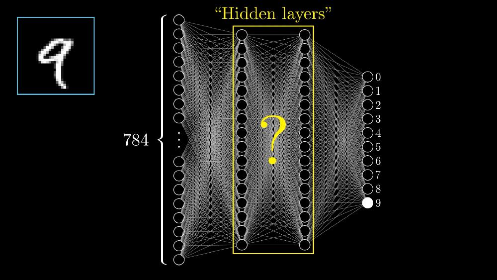
My first architecture (2 Hidden Layer NN) contained 2 hidden layers apart from input and output layer:

1. input layer of 784 neurons
2. Hidden Layer h1 of 50 neurons
3. Hidden layer h2 of 50 neurons
4. output layer of 10 neurons as we have 10 classes [0,9]

1
2
3
4
5
6
7
8

nn.Sequential(
	nn.Flatten(),
	nn.Linear(784,50),
	nn.ReLU(),
	nn.Linear(50,50),
	nn.ReLU(),
	nn.Linear(50,10)
)

And as this is a C class classification problem, I used CrossEntropy as loss function as its standard for classification problems. It penalizes the model more when it is confident about an incorrect class; less if it is less confident. And implicitly the first neuron of output layer represents 0, 2nd neuron represents 1, and so on… because cross entropy function takes 0 indexed class indices. So it all perfectly aligns without any need for remapping of training labels data.

Also, used Adam optimizer to update weights based on gradient found by backpropogation using loss function.

Adam optimizer (Adaptive Moment Estimation) efficiently adjusts the learning rates during training (dynamic learning rate). It works well with large datasets and complex models as it efficiently uses memory and adapts the LR for each parameter automatically.

Tweaking with training parameters

Version 1, 2 and 3

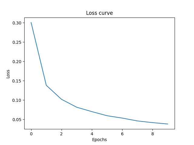
First I trained the model using 10 epochs, and accuracy was 97.24.

1
2
3
4
5
6
7
8

"model_type": "2_HL_NN_v1",
"test_accuracy": 97.24,
"train_accuracy": 99.13166666666666,
"final_train_loss": 0.038342890108324354,
"epochs": 10,
"batch_size": 50,
"learning_rate": 0.001,
"optimizer": "Adam"

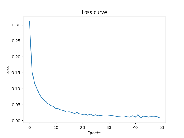
I then tried to increase the epochs to 50 to see the results:

1
2
3
4
5
6
7
8

"model_type": "2_HL_NN_v2",
"test_accuracy": 97.25,
"train_accuracy": 99.68166666666667,
"final_train_loss": 0.00926818358560228,
"epochs": 50,
"batch_size": 50,
"learning_rate": 0.001,
"optimizer": "Adam"

As you can see, the model performed slightly better on both the training and test datasets.

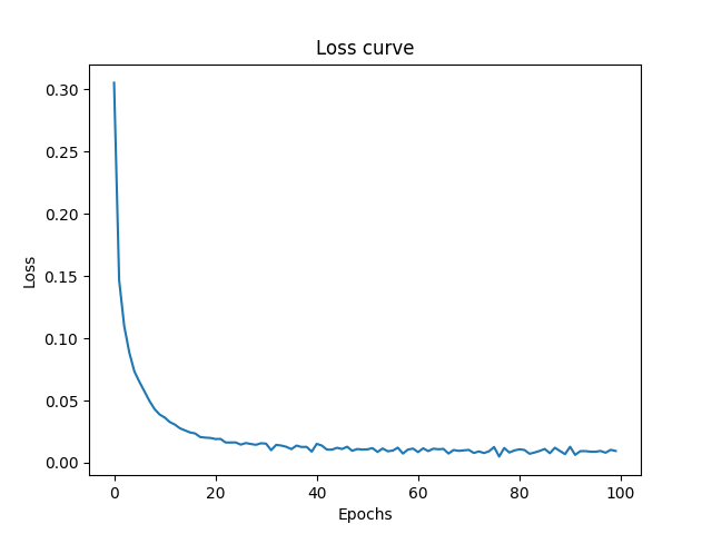
On 100 epochs the model performed substantially better

1
2
3
4
5
6
7
8

"model_type": "2_HL_NN_v3",
"test_accuracy": 97.5,
"train_accuracy": 99.81833333333333,
"final_train_loss": 0.009459313936198182,
"epochs": 100,
"batch_size": 50,
"learning_rate": 0.001,
"optimizer": "Adam"

If keep increasing that it starts overfitting and starts performing bad on the test dataset as we see later in the blog.

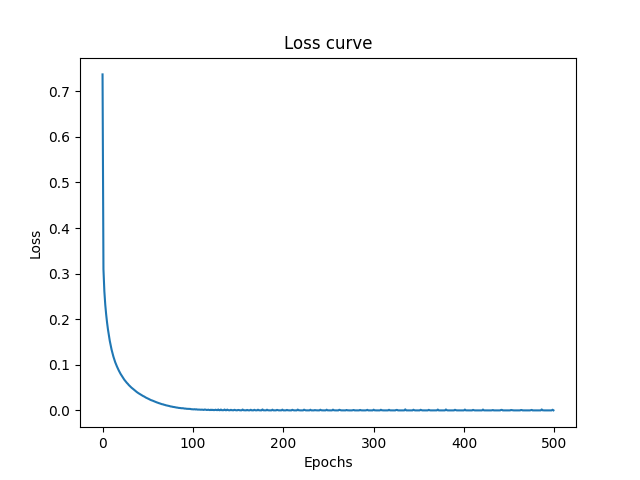
Loss Curves: As you can see, more epochs gave the model more iterations to update its weights properly, and hence it navigates closer to the global minima. The jaggy part of the curve shows the points where the model navigates to an uphill position due to momentum (learning rate) but in the next iteration comes back down the hill towards the minima. Note that this is just a simplification of the $N$-dimensional space onto 3 dimensions for understanding.

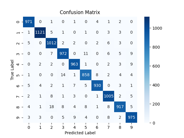
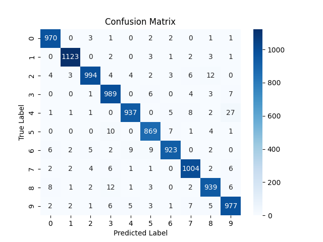
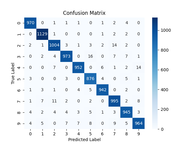
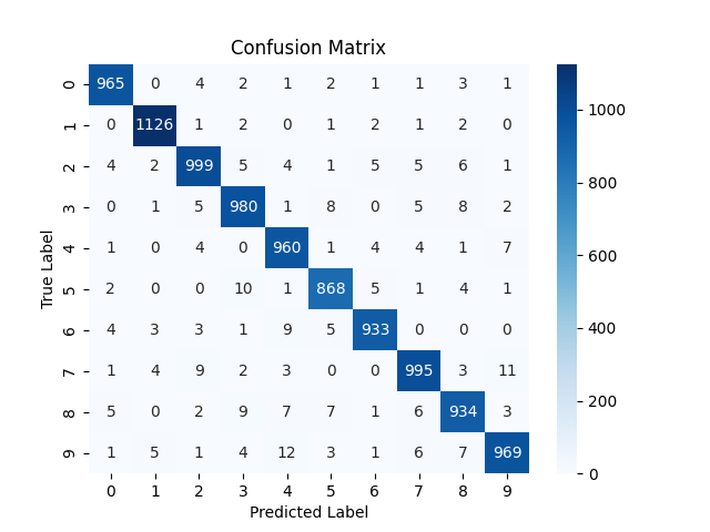
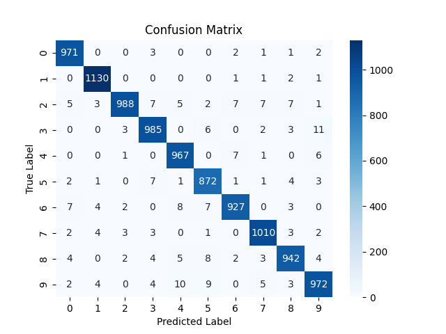
As you can see the model shows increase in positive classification rates (diagonals). Also there is decrease in confusion (wrong classification of some digits) although for some digits it increased a bit.

NOTE: the confusion matrix is based on the testing results on 10,000 test images.

Version 4

Now I increased the learning rate, which means the optimizer will make more bigger steps, meaning more momentum. In some cases this helps because it can potentially move past a local minima due to momentum. But in some cases it may overshoot the global minima and prevent the model from settling around the minima, causing it to constantly juggle back and forth on the valley and hill. In this case, the accuracy decreased to 95%, which means it failed to settle on the minima.

1
2
3
4
5
6
7
8

"model_type": "2_HL_NN_v4",
"test_accuracy": 95.29,
"train_accuracy": 97.22666666666667,
"final_train_loss": 0.12517643355588917,
"epochs": 100,
"batch_size": 50,
"learning_rate": 0.01,
"optimizer": "Adam"

Both training and test accuracy decreased. Loss curve never settles, it is very “jaggy” due to reasons stated above.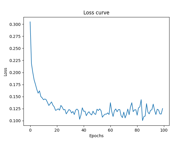

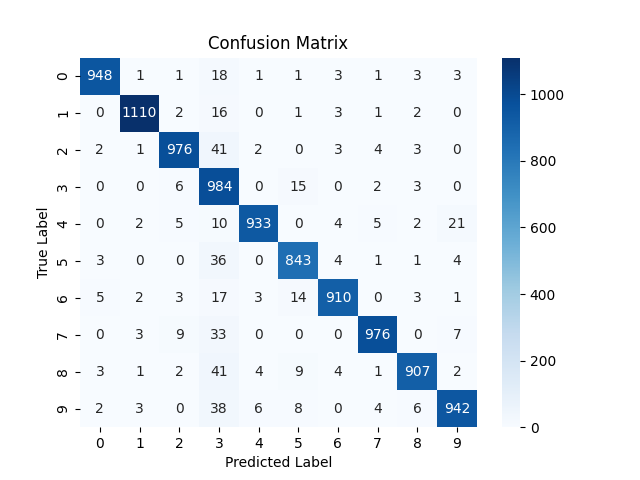
Confusion increased overall. One interesting observation is the column of digit 3. The model consistently predicted a number as a 3 when it was not actually a 3. The possible reasons might be:

• 3 has much overlap in pixels with other digits; mainly, the bottom-right curve overlaps with 5, 6, 8, 9, and 0, and the top-right curve overlaps with that of 2. So there is a lot of common area between 3 and other numbers. As the learning rate was higher, the model failed to learn the fine differentiating factors that make a 3 unique from all those. So whenever it sees those curves, it defaults to 3.
• Or maybe due to the high learning rate, the model learned that whenever it is uncertain, the safest bet is to predict 3 to minimize loss.

Version 5

Now I decreased the learning rate to 0.0001, and now the train accuracy reached 100%. However, compared to the 97.5% testing accuracy of model 2_HL_NN_v3, this model had a bit lower testing accuracy. The change is very small, so I can’t figure out the exact reason. Two possible reasons might be:

• Overfitting on the training dataset. As it settled heavily on the minima of the training landscape, it learned slightly less of the logical relationships and just tried to fit the training dataset.
• The second reason I think of is randomness. Because the Neural Network is initialized randomly before training begins, there is always a slight difference in output. I should have used seed for my network to be reproducible. But anyways, I am fine with that :) as the change is not substantial; only a 0.06% decrease.

1
2
3
4
5
6
7
8

"model_type": "2_HL_NN_v5",
"test_accuracy": 97.44,
"train_accuracy": 100.0,
"final_train_loss": 0.002149901499879737,
"epochs": 100,
"batch_size": 50,
"learning_rate": 0.0001,
"optimizer": "Adam"

However the learning curve was very SMOOTH as it should be due to small steps of optimizer.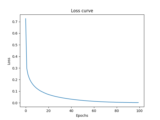

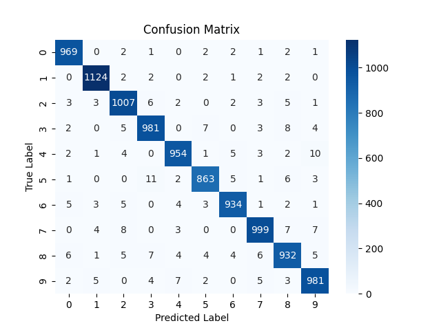
From now on I have kept the learning at 0.0001.

Version 6

I increased the epochs to 500. And yes, it overfitted to the training dataset. It achieved 100% train accuracy and 97.29% test accuracy. The test accuracy decreased. The final train loss is much lower due to the large no. of iterations.

1
2
3
4
5
6
7
8

"model_type": "2_HL_NN_v6",
"test_accuracy": 97.29,
"train_accuracy": 100.0,
"final_train_loss": 0.00015822308043662544,
"epochs": 500,
"batch_size": 50,
"learning_rate": 0.0001,
"optimizer": "Adam"

Version 7

Now resetting the epochs to 50, I increased the batch size to 1000. And oops… the test and training accuracy came down to 95.5%!

1
2
3
4
5
6
7
8

"model_type": "2_HL_NN_v7",
"test_accuracy": 95.56,
"train_accuracy": 95.9,
"final_train_loss": 0.14624120245377223,
"epochs": 50,
"batch_size": 1000,
"learning_rate": 0.0001,
"optimizer": "Adam"

The possible reasons:

• As the batch size increased, the number of weight updates per epoch reduced from 1200 to just 60. Combining this with the low learning rate of 0.0001 and only 50 epochs, the model didn’t get sufficient time to properly update the weights to descend to the global minima. (As both train and test accuracy decreased, this is the main reason; if only test accuracy had decreased, it would mean overfitting.) The model did not converge properly in those 50 epochs.

• Also, a large batch size strips away the noise inherent in smaller batch sizes. Because of the large size, on average the noise gets minimized as there will be more perfect training images compared to noisy ones. That means a loss of regularization noise. Sometimes this noise helps the optimizer escape sharp local minima that generalize poorly.

• Adam relies on the variance across batches to adapt the dynamic learning rates of neurons effectively. When the batch size is 1000, the gradients are so smoothed out that the variance between batches falls down. Adam’s adaptive mechanisms become much less effective, and it essentially behaves like standard gradient descent.

The most plausible reason I think is the first one. Actually, when you increase the batch size, you should also increase the learning rate. This is the Linear Scaling Rule:

When multiplying the mini-batch size by a factor in deep learning, the learning rate should also be multiplied by that factor to maintain stable training.

You can read the Linear Scaling Rule in the paper Accurate, Large Minibatch SGD: Training ImageNet in 1 Hour on arxiv paper

Loss Curve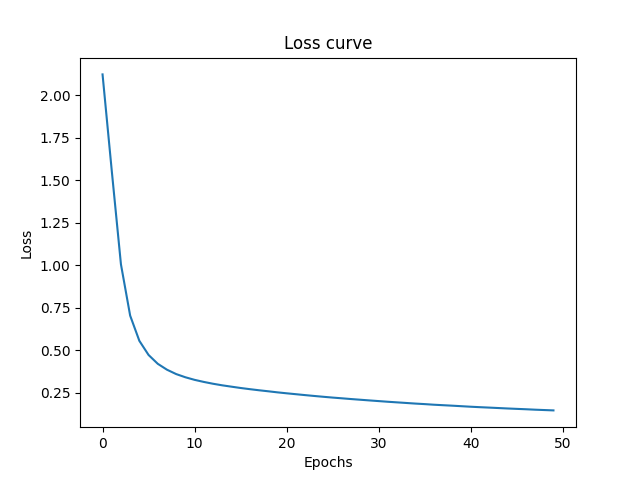

As you can see the curve had still not reached the plateau, when the training got finished.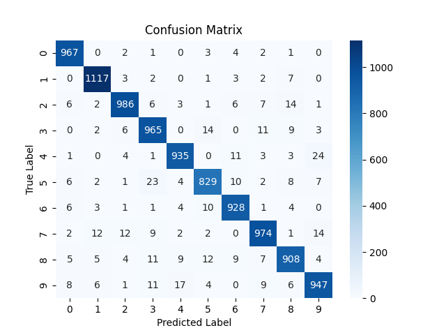

Version 8

Reduced batch size to 1. Which is essentially : no batching. Pure Stochastic gradient descent. And yeah this gave the highest testing accuracy of 97.64% (so far, we have better later).

1
2
3
4
5
6
7
8

"model_type": "2_HL_NN_v7",
"test_accuracy": 97.64,
"train_accuracy": 99.89333333333333,
"final_train_loss": 0.005643973710057734,
"epochs": 50,
"batch_size": 1,
"learning_rate": 0.0001,
"optimizer": "Adam"

That’s because compared to batch size of 100 or 1000, it got an exponentially higher number of weight updates: 60,000 weight updates per epoch, or 3 million updates in full training. It’s brute force! It got significantly more steps to traverse the loss landscape. This is also visible in terms of actual training time: it took around 50 minutes in total to train this model, which is much longer than the 5-10 minutes for other runs, even though this dataset is relatively tiny compared to other datasets.

Did I use a GPU then? Yes, I used Google Colab’s T4 GPU compute. But it’s of no use in this case, because a batch size of 1 essentially does the training sequentially rather than using its full parallelization power. It’s like training on a CPU or even worse if we take into account the setup overhead of the GPU for computation (like transferring data from CPU RAM to GPU VRAM), which in case of large batches gets spread over all samples, which compared to time advantage from parallelization makes it look tiny.

So for training models, a batch size of 1 is terrible in most cases (unless a single sample requires massive matrix computations).

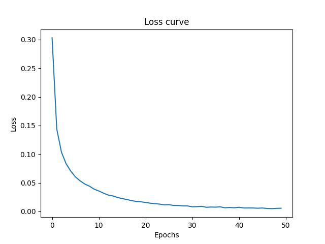
NOTE: MNIST dataset does not seem to be that noisy, otherwise the loss curve would have been very jaggy for batch size of 1 for the reasons already discussed above.

3 Hidden Layer NN

 1
 2
 3
 4
 5
 6
 7
 8
 9
10

Sequential(
    nn.Flatten(),
    nn.Linear(784,50),
    nn.ReLU(),
    nn.Linear(50,50),
    nn.ReLU(),
    nn.Linear(50,50),
    nn.ReLU(),
	nn.Linear(50,10)
)

Version 1

Got no substantial advantage.

1
2
3
4
5
6
7
8

"model_type": "3_HL_NN_v1",
"test_accuracy": 97.31,
"train_accuracy": 99.56333333333333,
"final_train_loss": 0.024630995460490038,
"epochs": 50,
"batch_size": 50,
"learning_rate": 0.0001,
"optimizer": "Adam"

However, the loss curve shows that it didn’t reach a plateau by the end of training. I retrained it for 100 epochs but got no substantial increase in accuracy.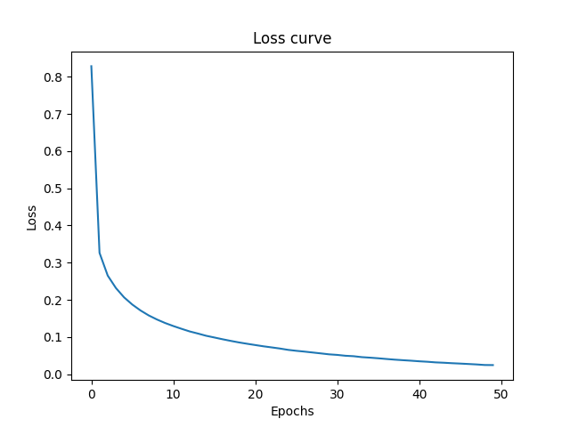

So it seems increasing the number of layers did no better than 2 layers. Hence, it reminds us that “deeper is not always better” in deep learning. Especially for a simple dataset like MNIST, stacking layers is not beneficial as such. The 2-layer network is already capable of approximating a function to solve this problem, mapping a 784-dimensional vector to a 10-dimensional vector. More layers are needed only when we have to approximate a much more complex function like image classification on the ImageNet dataset using a CNN, with each layer learning some feature like texture, edges, etc.

In our case, adding more layers makes the model learn very fine-grained pixel settings and noise, which is not necessary at all. The loss landscape becomes much more complex.

Even a single layer network gave fair results. 97.27% test accuracy and 99.97% train accuracy.

1
2
3
4
5
6
7
8

"model_type": "1_HL_NN_v1",
"test_accuracy": 97.27,
"train_accuracy": 99.97666666666667,
"final_train_loss": 0.00654870391087267,
"epochs": 100,
"batch_size": 50,
"learning_rate": 0.0001,
"optimizer": "Adam"

Version 2

I tried to experiment with Sigmoid Activation function instead of ReLU. But as expected, it did worse.

1
2
3
4
5
6
7
8

nn.Flatten(),
nn.Linear(784,50),
nn.Sigmoid(),
nn.Linear(50,50),
nn.Sigmoid(),
nn.Linear(50,50),
nn.Sigmoid(),
nn.Linear(50,10)

1
2
3
4
5
6
7
8

"model_type": "3_HL_NN_v2",
"test_accuracy": 95.93,
"train_accuracy": 98.71666666666667,
"final_train_loss": 0.06427663042986144,
"epochs": 50,
"batch_size": 50,
"learning_rate": 0.0001,
"optimizer": "Adam"

The test accuracy decreased to 95.93%

Sigmoid Function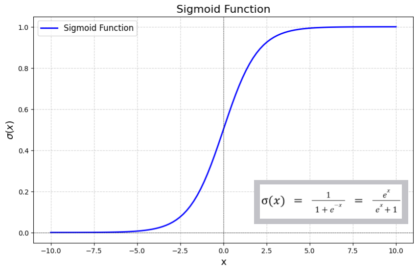

Most of the values accumulate around 1 and 0 and not in-between, and the gradient at those points tends to 0. Hence, the weights have a very small update magnitude. The derivative $\sigma'(z) = \sigma(z)(1 - \sigma(z))$ has an absolute maximum of $0.25$. In a 3-hidden-layer architecture, the chain rule multiplies these fractions backward (e.g., $0.25^3 = 0.0156$ in the best case scenario), mathematically preventing the earliest layers from receiving a meaningful learning signal.

Also, if the neuron’s preactivation values are strongly positive or negative, the curve flattens completely, making the gradient zero. Hence, it FREEZES the neurons and restricts learning.

This is commonly called the vanishing gradient problem.

To handle this, we usually use two approaches:

1. Proper Weight Initialisation: Xavier Initialisation (Glorot Initialisation). It keeps the signal variance consistent across layers, preventing the weights from being so large or small that the sigmoid saturates (flattens out) at 0 or 1.

2. Input Scaling: Which we already did! Making input data normalised or standardised (typically scaled to a range like [0, 1] or [-1, 1]) prevents saturation. If inputs are too large, the function immediately enters the flat regions where the gradient is nearly zero, effectively “killing” the neuron’s ability to learn.

ReLU Function: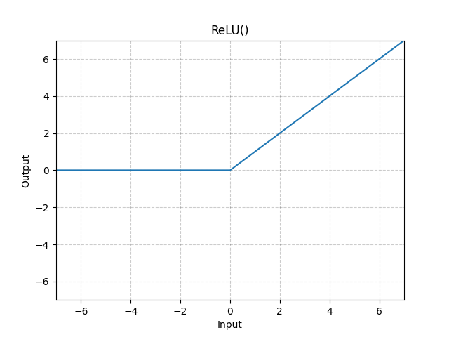

The learning signal does not diminish as it travels back to the earliest layers, completely eradicating the vanishing gradient problem that plagues sigmoid ($0.25 \times 0.25 \times 0.25$). Also there is no accumulation towards 1 on positive side, due to linear function.

However on negative side its complete 0. If a large gradient update pushes a neuron’s weights such that $z \le 0$ for the entire dataset, the neuron outputs 0, and gradient = 0. The weights can never update again. The neuron is mathematically dead.

In a deep network with a high learning rate, up to 40% of the ReLU network can silently die during early training, turning massive architecture into a highly constrained, inefficient model.

Version 3

Reducing number of neurons

 1
 2
 3
 4
 5
 6
 7
 8
 9
10

nn.Sequential(
    nn.Flatten(),
    nn.Linear(784,10),
    nn.ReLU(),
    nn.Linear(10,10),
    nn.ReLU(),
    nn.Linear(10,10),
    nn.ReLU(),
	nn.Linear(10,10)
),

1
2
3
4
5
6
7
8

"model_type": "3_HL_NN_v3",
"test_accuracy": 93.56,
"train_accuracy": 94.32666666666667,
"final_train_loss": 0.19906658599463603,
"epochs": 50,
"batch_size": 50,
"learning_rate": 0.0001,
"optimizer": "Adam"

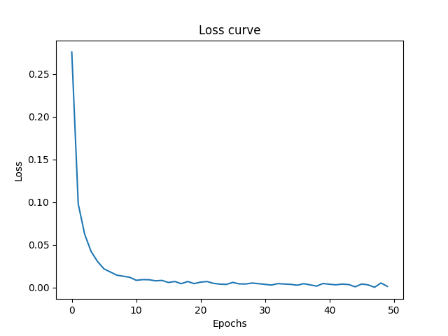
The Test Accuracy decreased. Also observing the loss curve, it’s clear that the model has ample time for learning, as it started to reach a plateau around 0.2.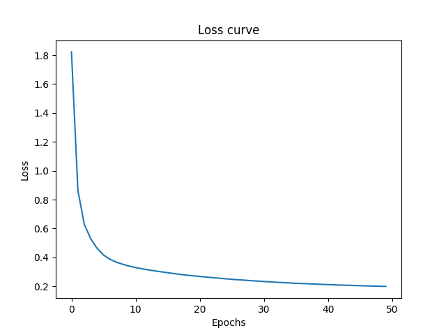

It’s severe underfitting. So the issue is that fewer neurons failed to capture the nuances of the $28 \times 28 = 784$ pixels. By mapping the input layer directly from 784 dimensions down to just 10, we have a tight bottleneck for information.

The first hidden layer of a neural network is responsible for extracting low-level features (like strokes or edges). To classify 10 distinct digits, the network needs to hold enough combinations of these strokes in its active memory. When we compress 784 pixels into a 10-dimensional vector, the projection matrix $W \in \mathbb{R}^{10 \times 784}$ forces the network to discard massive amounts of variance. This shows that it is mathematically impossible to linearly separate the complex, entangled features of the MNIST dataset within a space that is only 10 dimensions wide without losing critical distinguishing information.

Also, the uniform number of neurons across layers poses a problem. Because the layers never expand, the network can never recover or recombine features into a higher-dimensional space to make them linearly separable before the final classification.

Version 4

Increasing neurons to 100. And yeah the accuracy increased to 97.81.

1
2
3
4
5
6
7
8

nn.Flatten(),
nn.Linear(784,100),
nn.ReLU(),
nn.Linear(100,100),
nn.ReLU(),
nn.Linear(100,100),
nn.ReLU(),
nn.Linear(100,10)

1
2
3
4
5
6
7
8

"model_type": "3_HL_NN_v4",
"test_accuracy": 97.81,
"train_accuracy": 99.94,
"final_train_loss": 0.0022639009931902385,
"epochs": 50,
"batch_size": 50,
"learning_rate": 0.0001,
"optimizer": "Adam"

Version 5

Now increased the number of neurons to 1000 (more than 784 input dimensions), and yeah accuracy increased to 98.32%, the best model I got in this whole experiment.

 1
 2
 3
 4
 5
 6
 7
 8
 9
10

nn.Sequential(
    nn.Flatten(),
    nn.Linear(784,1000),
    nn.ReLU(),
    nn.Linear(1000,1000),
    nn.ReLU(),
    nn.Linear(1000,1000),
    nn.ReLU(),
    nn.Linear(1000,10)
)

1
2
3
4
5
6
7
8

"model_type": "3_HL_NN_v5",
"test_accuracy": 98.32,
"train_accuracy": 99.915,
"final_train_loss": 0.0014889567906926087,
"epochs": 50,
"batch_size": 50,
"learning_rate": 0.0001,
"optimizer": "Adam"

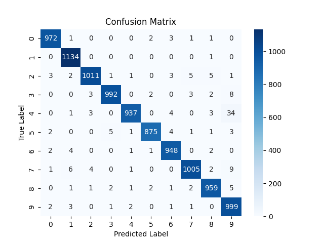
However, there is unusually high confusion between 9 and 4 compared to previous models. This suggests the model successfully approximated the function for all other digits, except 4 and 9. A CNN would help here.

The increase in accuracy may be due to capturing more detailed features and relationships from the 784 pixels to make a decision, but it’s not purely that. It is also a slight overfitting. Because as you increase the number of neurons, you give more space for the model to just memorize the data. But the testing accuracy increased anyway. This is likely an example of Benign Overfitting. (Though i doubt it in our case as its just a simple problem - MNIST, and not an complex network/problem or LLM)

Benign overfitting is a phenomenon in machine learning where a model perfectly fits its training data (achieving zero training error), including any noise or random errors, yet still manages to generalize and perform with high accuracy on new, unseen data. This discovery challenges the “classical statistical wisdom” of the bias-variance tradeoff, which typically suggests that such extreme fitting leads to poor predictive performance.

Actually, I had never read about this before these experiments. I just increased the number of neurons out of curiosity and found it unusual that the test error actually decreased instead of showing signs of overfitting, and then went on to do some research on the topic. But as it turned out, it is already published :( sad life.

This actually is a highly active and “hot” field in deep learning theory, as it provides the theoretical backbone for why modern overparameterized models; like LLMs; work so well. This behavior is the exact setup that gave birth to the Modern Deep Learning Theory.

It is hot in the sense that earlier work was focused only on Linear regression or simple kernels and not Neural Networks like this. It is just that recent high-impact papers (2024–2025) are finally bridging the gap to deep ReLU networks and non-linear settings.

The core idea is that in highly complex, over-parameterized models (like deep neural networks), the model’s prediction rule can be split into two parts: 

A Simple Component: A low-complexity part that captures the actual underlying signal or pattern in the data.

A “Spiky” Component: A high-complexity part that “absorbs” the noise at specific training points without affecting the model’s overall shape or predictions elsewhere. arXiv

It generalized despite of overfitting.

Actually we can plot a curve of number of neurons and test errors. Which would show the phenomenon of Double Descent which was studied by Mikhail Belkin in 2018 and then in 2019 by OpenAI researches as Deep Double Descent

Double descent is a machine learning phenomenon where a model’s test error first decreases, then increases, and finally decreases again as model complexity or training time grows.

Deep Double descent (OpenAI) - they extended it to Deep and complex neural networks beyond normal ML models just like I did in my case for MNIST dataset. OpenAI did it for ResNet18.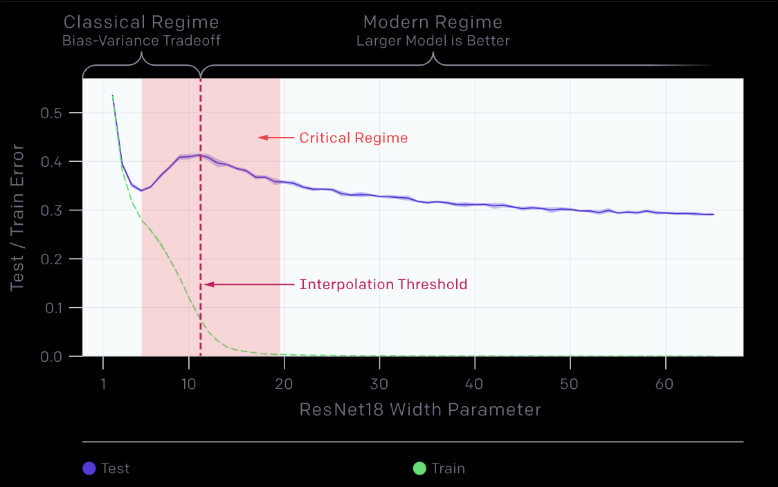

Also this network surely has many redundant neurons.

NOTE: This model took 34 minutes to train due to the high number of neurons. So brute-forcing didn’t give significant returns: an exponential increase in the number of neurons gave decaying returns.

100 neurons : 97.8 1000 neurons: 98.32

Let’s see what CNN can achieve compared to these soon.

References